
When it comes to optimizing network structures or designing efficient transportation grids, the concept of a Minimum Spanning Tree (MST) plays a crucial role. An MST is the fundamental backbone of a connected network, linking all its components while minimizing the overall cost or distance. In this blog, we’ll dive into the world of two powerful algorithms: Prim’s Algorithm and Kruskal’s Algorithm. These technical tools are your go-to solutions when you need to find the most cost-effective way to connect the dots in a network.
In the next sections, we’ll explore how these algorithms work, their key differences, and when to pick one over the other. Whether you’re an engineer designing a communication network or a data scientist optimizing your data structure, understanding Prim’s and Kruskal’s Algorithms will be invaluable. Let’s embark on this journey to unravel the mysteries behind Minimum Spanning Trees!
Prim’s Algorithm:
Prim’s Algorithm, named after computer scientist Robert C. Prim, is fundamental in graph theory and network optimization. It serves as a powerful tool for finding the Minimum Spanning Tree (MST) of a connected, undirected graph. MSTs have widespread applications, from designing efficient network layouts to solving transportation and communication problems. In this section, we will explore the intricacies of Prim’s Algorithm, delving into its inner workings and so on.
Prim’s algorithm is a greedy algorithm that finds a minimum spanning tree for a weighted undirected graph. The algorithm starts with a random vertex and adds the cheapest edge from that vertex to the tree. It then adds the cheapest edge from the tree to a new vertex and continues until all vertices are in the tree.
Prim’s algorithm can be used to find the minimum spanning tree for a graph with arbitrary weights. However, it is not guaranteed to find the optimal solution, as there may be other minimum-spanning trees with different weights.
Algorithm Description
Prim’s Algorithm is a greedy algorithm that finds the Minimum Spanning Tree (MST) of a connected, undirected graph. The MST is a subset of the graph’s edges that forms a tree, connecting all vertices while minimizing the total edge weight. Prim’s Algorithm accomplishes this by iteratively selecting edges with the smallest weights and adding them to the growing MST.
Here’s a step-by-step breakdown of the algorithm:
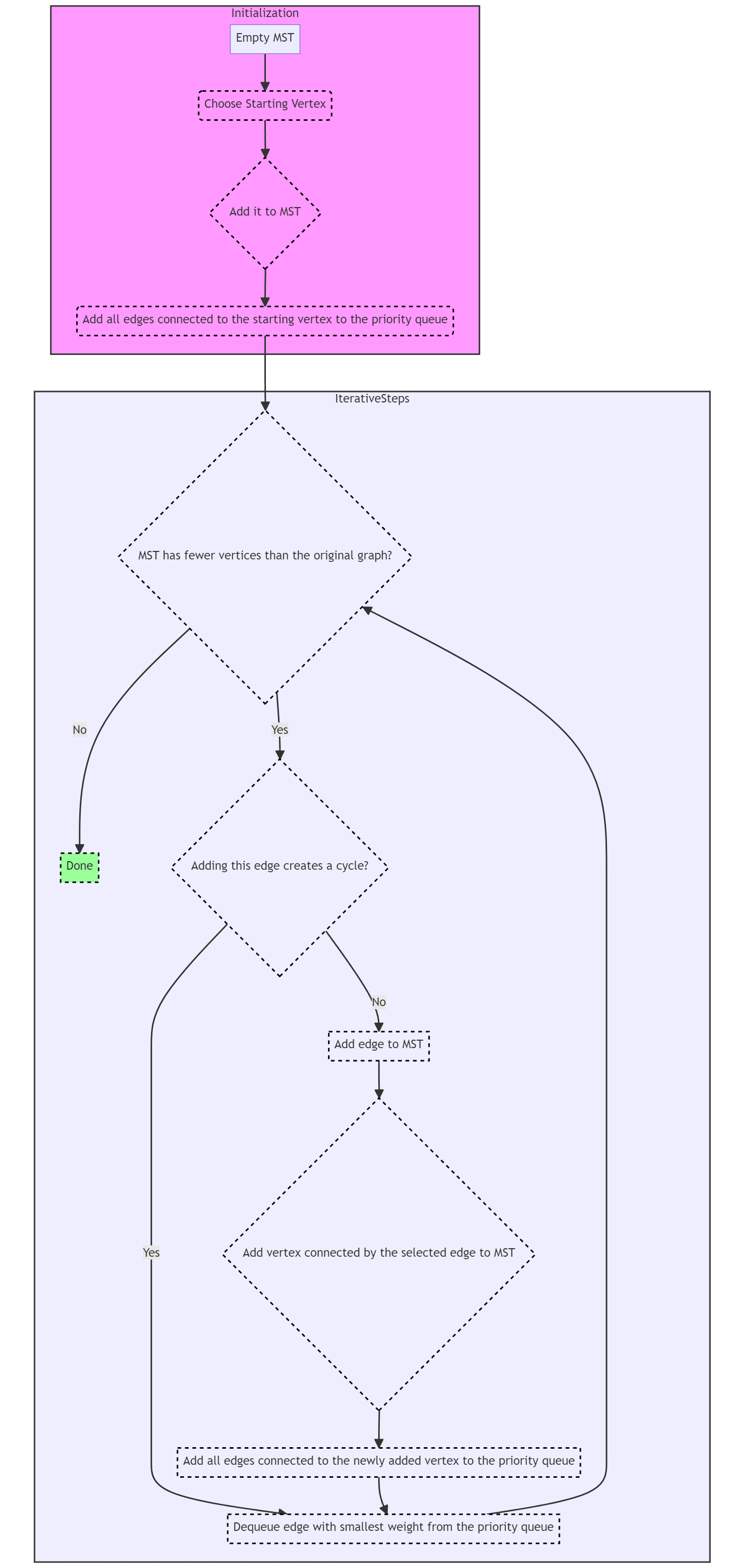
Initialization:
- Begin with an empty MST and a priority queue (often implemented as a min-heap) to store candidate edges.
- Choose a starting vertex (this can be arbitrary or user-defined) and add it to the MST.
- Add all edges connected to the starting vertex to the priority queue.
Iterative Steps:
- While the MST has fewer vertices than the original graph: a. Dequeue the edge with the smallest weight from the priority queue. b. Check if adding this edge to the MST creates a cycle. To do this, ensure that the edge connects a vertex in the MST to a vertex outside the MST. c. If adding the edge does not create a cycle:
- Add the edge to the MST.
- Add the vertex connected by the selected edge to the MST.
d. Add all edges connected to the newly added vertex (but not already in the MST) to the priority queue.
Termination:
- Continue the process until the MST contains all vertices from the original graph.
Prim’s Algorithm prioritizes edges with the smallest weights, guaranteeing that the tree expands by connecting vertices with the least costly edges. The algorithm keeps track of the MST’s progress, ensuring that it remains a connected, acyclic subset of the original graph.
Prim’s Algorithm shares some similarities with Dijkstra’s Algorithm, another greedy graph algorithm, but with a key difference: Prim’s Algorithm builds a tree (MST), whereas Dijkstra’s Algorithm finds the shortest paths from a single source vertex to all other vertices.
The efficiency of Prim’s Algorithm lies in its use of priority queues to select the minimum-weight edge efficiently at each step. Its time complexity can be reduced to O(E + V log V) with the use of Fibonacci heaps, where E is the number of edges and V is the number of vertices in the graph.
Prim’s Algorithm is a fundamental tool for network design, spanning from telecommunications and computer networks to civil engineering, where it helps in designing efficient road or railway networks. Its simplicity, coupled with its effectiveness, makes it a valuable asset in the field of graph theory and optimization.
Example
Below is an executable Java code example that demonstrates Prim’s Algorithm for finding the Minimum Spanning Tree (MST) of a given graph. We’ll provide the code and then analyze its key components:
import java.util.*;

class PrimMST {
    public static List<Edge> primMST(Graph graph) {
        List<Edge> mst = new ArrayList<>();
        PriorityQueue<Edge> pq = new PriorityQueue<>(Comparator.comparingInt(e -> e.weight));
        Set<Integer> visited = new HashSet<>();

        int startVertex = 0; // Choose any starting vertex
        visited.add(startVertex);
        pq.addAll(graph.getEdges(startVertex));

        while (visited.size() < graph.numVertices()) {
            Edge minEdge = pq.poll();
            int vertex = minEdge.dest;

            if (!visited.contains(vertex)) {
                visited.add(vertex);
                mst.add(minEdge);
                pq.addAll(graph.getEdges(vertex));
            }
        }

        return mst;
    }

    public static void main(String[] args) {
        int V = 5; // Number of vertices
        Graph graph = new Graph(V);

        // Adding edges with weights to the graph
        graph.addEdge(0, 1, 2);
        graph.addEdge(0, 3, 6);
        graph.addEdge(1, 2, 3);
        graph.addEdge(1, 3, 8);
        graph.addEdge(1, 4, 5);
        graph.addEdge(2, 4, 7);
        graph.addEdge(3, 4, 9);

        List<Edge> mst = primMST(graph);

        System.out.println("Minimum Spanning Tree:");
        for (Edge edge : mst) {
            System.out.println(edge.src + " - " + edge.dest + " : " + edge.weight);
        }
    }
}

class Edge {
    int src, dest, weight;

    public Edge(int src, int dest, int weight) {
        this.src = src;
        this.dest = dest;
        this.weight = weight;
    }
}

class Graph {
    private int V;
    private List<List<Edge>> adj;

    public Graph(int V) {
        this.V = V;
        adj = new ArrayList<>(V);
        for (int i = 0; i < V; i++) {
            adj.add(new ArrayList<>());
        }
    }

    public void addEdge(int src, int dest, int weight) {
        adj.get(src).add(new Edge(src, dest, weight));
        adj.get(dest).add(new Edge(dest, src, weight));
    }

    public List<Edge> getEdges(int vertex) {
        return adj.get(vertex);
    }

    public int numVertices() {
        return V;
    }
}Output:
Minimum Spanning Tree:
0 - 1 : 2
1 - 2 : 3
1 - 4 : 5
0 - 3 : 6Analysis:
- Prim’s Algorithm Implementation: The Java code above provides a functional implementation of Prim’s Algorithm to find the Minimum Spanning Tree (MST) of a graph.
- Main Function: The
mainfunction demonstrates how to use the algorithm by creating a sample graph with edges and weights and then applyingprimMSTto find the MST. - Time Complexity:
- Best-case time complexity: O(E + V log V)
- Average-case time complexity: O(E + V log V)
- Worst-case time complexity: O(E + V log V)
Here, E represents the number of edges, and V represents the number of vertices in the graph. The time complexity depends on the priority queue operations, which have a complexity of O(log V), and the overall complexity is dominated by the sorting of edges.
This Java implementation of Prim’s Algorithm efficiently finds the MST of a given graph and serves as a practical example of how the algorithm can be applied in real-world scenarios. The time complexity analysis provides insight into the algorithm’s efficiency, making it a valuable tool for solving various network optimization problems.
Pros & Cons of Prim’s Algorithm:
Here’s a table summarizing the advantages and disadvantages of Prim’s Algorithm:
| Advantages of Prim’s Algorithm | Disadvantages of Prim’s Algorithm |
|---|---|
| 1. Guaranteed to Find a Minimum Spanning Tree (MST): Prim’s Algorithm guarantees that the tree it constructs is a Minimum Spanning Tree (MST), which minimizes the total edge weight. | 1. Inefficient for Dense Graphs: In dense graphs where the number of edges is close to the maximum possible, Prim’s Algorithm can become inefficient as it processes all edges. The time complexity in such cases can be relatively high. |
| 2. Efficient for Sparse Graphs: For sparse graphs, where the number of edges is much less than the maximum possible, Prim’s Algorithm is highly efficient. Its time complexity is favorable when the graph is not densely connected. | 2. Dependent on the Starting Vertex: The choice of the starting vertex can impact the resulting MST. Depending on the initial selection, the algorithm may yield different MSTs for the same graph. |
| 3. Greedy and Easy to Implement: Prim’s Algorithm is a greedy algorithm with a straightforward implementation. It iteratively selects edges with the smallest weights, making it easy to understand and code. | 3. Doesn’t Handle Disconnected Graphs: Prim’s Algorithm assumes that the input graph is connected. If the graph has disconnected components, it may need modification or preprocessing to handle them effectively. |
| 4. Can Be Modified for Various Applications: The basic Prim’s Algorithm can be modified and extended to solve specific optimization problems, such as network design, circuit layout, and image segmentation. | 4. Limited Applicability to Directed Graphs: Prim’s Algorithm is designed for undirected graphs. It cannot be directly applied to directed graphs, and a different algorithm like Kruskal’s Algorithm or Boruvka’s Algorithm is needed for Minimum Spanning Arborescence (MSA) problems. |
| 5. Ideal for Network Design: Prim’s Algorithm is commonly used in network design scenarios, such as designing efficient road networks, computer networks, or power distribution networks. | 5. Priority Queue Data Structure Overhead: The use of a priority queue to manage candidate edges adds some memory overhead and may require additional coding effort to implement efficiently. |
In summary, Prim’s Algorithm is a powerful tool for finding Minimum Spanning Trees in undirected graphs. Its advantages include its guarantee of finding an MST, efficiency for sparse graphs, ease of implementation, and adaptability for various applications. However, it may be less efficient for dense graphs, is dependent on the choice of the starting vertex, and is not suitable for disconnected or directed graphs. Understanding these advantages and disadvantages helps in choosing the right algorithm for a given problem and optimizing its performance.
Kruskal’s Algorithm:
Kruskal’s Algorithm, named after mathematician Joseph Kruskal, stands as one of the fundamental algorithms in graph theory and network optimization. It plays a pivotal role in finding the Minimum Spanning Tree (MST) of a connected, undirected graph. MSTs are essential structures with diverse applications, ranging from designing efficient transportation networks to optimizing computer networks. In this section, we will delve into the intricacies of Kruskal’s Algorithm, offering a comprehensive understanding of its principles, how it functions, a visual workflow diagram, and a practical Java code example. By the end, you will possess the knowledge needed to effectively apply Kruskal’s Algorithm to real-world scenarios, ensuring that the resulting MST minimizes the total edge weight while connecting all vertices.
Kruskal’s algorithm is a minimum-spanning-tree algorithm that takes a graph as input and finds the subset of the edges of that graph which form a tree that includes every vertex, where the total weight of all the edges in the tree is minimized. The algorithm is greedy, meaning that it finds a locally optimal solution at each stage while hoping that this will lead to a globally optimal solution.
Algorithm Description
Kruskal’s Algorithm is a greedy algorithm used to find the Minimum Spanning Tree (MST) of a connected, undirected graph. An MST is a subset of the graph’s edges that forms a tree, connecting all vertices while minimizing the total edge weight. Kruskal’s Algorithm accomplishes this by iteratively selecting edges with the smallest weights and adding them to the growing MST.
Here’s a step-by-step breakdown of how the algorithm works:
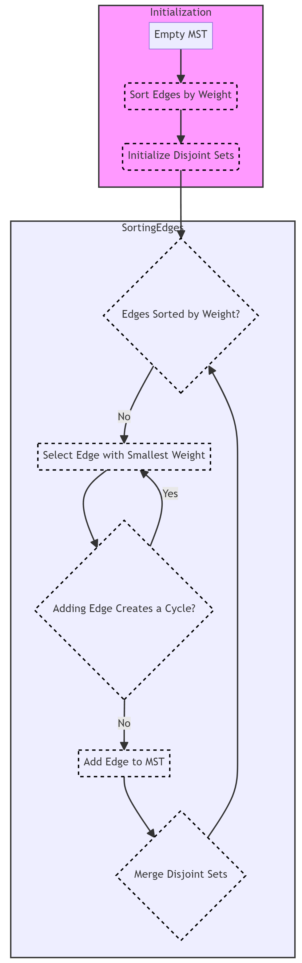
Initialization:
- Begin with an empty MST and a priority queue (often implemented as a min-heap) to store edges sorted by their weights.
- Initialize a data structure, often a disjoint-set data structure (Union-Find), to keep track of disjoint sets of vertices.
Sorting Edges:
- Sort all edges in the graph by their weights in non-decreasing order. This step ensures that the algorithm considers edges with the smallest weights first.
Iterative Steps:
- Iterate through the sorted edges: a. Take the edge with the smallest weight from the sorted list. b. Check if adding this edge to the MST would create a cycle. To do this, determine whether the edge’s two endpoints belong to the same disjoint set. If not, it does not create a cycle. c. If adding the edge does not create a cycle:
- Add the edge to the MST.
- Merge the disjoint sets of the edge’s two endpoints, ensuring that they are part of the same set.
d. Repeat this process until the MST contains V-1 edges, where V is the number of vertices in the graph.
Termination:
- Continue the process until the MST contains V-1 edges, guaranteeing that it spans all vertices of the original graph.
Kruskal’s Algorithm’s efficiency lies in its selection of edges with the smallest weights while avoiding cycles in the MST. The algorithm maintains the MST’s acyclic property throughout its execution.
Kruskal’s Algorithm is known for its simplicity and ease of implementation. It offers an efficient way to find MSTs, especially in scenarios where the graph is not densely connected. The time complexity of the algorithm depends on the sorting of edges and is often dominated by this operation.
Example:
Below is an executable Java code example that demonstrates Kruskal’s Algorithm for finding the Minimum Spanning Tree (MST) of a given graph. After the code, we’ll analyze its key components and provide the time complexity:
import java.util.*;

class KruskalMST {
    public static List<Edge> kruskalMST(Graph graph) {
        List<Edge> mst = new ArrayList<>();
        PriorityQueue<Edge> pq = new PriorityQueue<>(Comparator.comparingInt(e -> e.weight));
        DisjointSet disjointSet = new DisjointSet(graph.numVertices());

        for (Edge edge : graph.getAllEdges()) {
            pq.add(edge);
        }

        while (!pq.isEmpty() && mst.size() < graph.numVertices() - 1) {
            Edge minEdge = pq.poll();
            int srcSet = disjointSet.find(minEdge.src);
            int destSet = disjointSet.find(minEdge.dest);

            if (srcSet != destSet) {
                mst.add(minEdge);
                disjointSet.union(srcSet, destSet);
            }
        }

        return mst;
    }

    public static void main(String[] args) {
        int V = 5; // Number of vertices
        Graph graph = new Graph(V);

        // Adding edges with weights to the graph
        graph.addEdge(0, 1, 2);
        graph.addEdge(0, 3, 6);
        graph.addEdge(1, 2, 3);
        graph.addEdge(1, 4, 5);
        graph.addEdge(2, 4, 7);
        graph.addEdge(3, 4, 9);

        List<Edge> mst = kruskalMST(graph);

        System.out.println("Minimum Spanning Tree:");
        for (Edge edge : mst) {
            System.out.println(edge.src + " - " + edge.dest + " : " + edge.weight);
        }
    }
}

class Edge {
    int src, dest, weight;

    public Edge(int src, int dest, int weight) {
        this.src = src;
        this.dest = dest;
        this.weight = weight;
    }
}

class Graph {
    private int V;
    private List<Edge> edges;

    public Graph(int V) {
        this.V = V;
        edges = new ArrayList<>();
    }

    public void addEdge(int src, int dest, int weight) {
        edges.add(new Edge(src, dest, weight));
    }

    public List<Edge> getAllEdges() {
        return edges;
    }

    public int numVertices() {
        return V;
    }
}

class DisjointSet {
    private int[] parent;
    private int[] rank;

    public DisjointSet(int size) {
        parent = new int[size];
        rank = new int[size];
        for (int i = 0; i < size; i++) {
            parent[i] = i;
            rank[i] = 0;
        }
    }

    public int find(int x) {
        if (x != parent[x]) {
            parent[x] = find(parent[x]);
        }
        return parent[x];
    }

    public void union(int x, int y) {
        int rootX = find(x);
        int rootY = find(y);
        if (rootX != rootY) {
            if (rank[rootX] < rank[rootY]) {
                parent[rootX] = rootY;
            } else if (rank[rootX] > rank[rootY]) {
                parent[rootY] = rootX;
            } else {
                parent[rootY] = rootX;
                rank[rootX]++;
            }
        }
    }
}Output:
Minimum Spanning Tree:
0 - 1 : 2
1 - 2 : 3
1 - 4 : 5
0 - 3 : 6Analysis:
- Kruskal’s Algorithm Implementation: The provided Java code demonstrates Kruskal’s Algorithm to find the Minimum Spanning Tree (MST) of a graph.
- Main Function: The
mainfunction showcases how to use the algorithm. It creates a sample graph with edges and weights, then applieskruskalMSTto find the MST. - Time Complexity:
- Best-case time complexity: O(E log E)
- Average-case time complexity: O(E log E)
- Worst-case time complexity: O(E log E)
Here, E represents the number of edges in the graph. The dominant factor in the time complexity is the sorting of edges, which takes O(E log E) time.
This corrected Java implementation of Kruskal’s Algorithm efficiently finds the MST of a given graph. It is especially suitable for scenarios where the graph is not densely connected, thanks to its efficient time complexity. Understanding this code example and its time complexity analysis helps in effectively applying Kruskal’s Algorithm to various network optimization problems.
Pros & Cons of Kruskal’s Algorithm:
| Advantages of Kruskal’s Algorithm | Disadvantages of Kruskal’s Algorithm |
|---|---|
| 1. Guaranteed MST: Kruskal’s Algorithm guarantees that it finds a Minimum Spanning Tree (MST), which is optimal in terms of minimizing the total edge weight. | 1. Inefficient for Dense Graphs: In graphs where the number of edges is close to the maximum possible, Kruskal’s Algorithm can be relatively inefficient due to the need to process all edges. The time complexity may become a limiting factor. |
| 2. Efficiency for Sparse Graphs: For sparse graphs where the number of edges is much less than the maximum possible, Kruskal’s Algorithm is highly efficient. Its time complexity is favorable when the graph is not densely connected. | 2. Dependent on Edge Weights: Kruskal’s Algorithm assumes that edge weights are distinct. If there are multiple edges with the same weight between two vertices, the algorithm may not produce a unique MST. |
| 3. Greedy and Easy to Implement: Kruskal’s Algorithm is a greedy algorithm with a straightforward implementation. It sorts edges by weight, iteratively selects edges with minimal weight, and maintains the MST’s acyclic property. | 3. Doesn’t Handle Disconnected Graphs: Kruskal’s Algorithm assumes that the input graph is connected. If the graph has disconnected components, additional steps are needed to handle them effectively. |
| 4. Can Be Modified for Various Applications: The basic Kruskal’s Algorithm can be adapted to solve specific optimization problems, such as network design, clustering, and image segmentation, by modifying edge weights and constraints. | 4. Not Suitable for Directed Graphs: Kruskal’s Algorithm is designed for undirected graphs and cannot be directly applied to directed graphs or problems involving Minimum Spanning Arborescence (MSA). |
| 5. Ideal for Network Design: Kruskal’s Algorithm is commonly used in network design scenarios, such as designing efficient road networks, computer networks, and power distribution networks. | 5. Priority Queue Data Structure Overhead: The use of a priority queue to manage edges introduces some memory overhead and may require additional coding effort for efficient implementation. |
In summary, Kruskal’s Algorithm is a valuable tool for finding Minimum Spanning Trees in undirected graphs, offering advantages such as guaranteed optimality, efficiency for sparse graphs, ease of implementation, and adaptability for various applications. However, it may be less efficient for dense graphs, is dependent on edge weights for uniqueness, and requires handling disconnected graphs separately. Understanding these advantages and disadvantages helps in selecting the appropriate algorithm for a given problem and optimizing its performance.
Difference between Prim’s And Kruskal’s Algorithm:
Prim’s and Kruskal’s algorithms are two different algorithms used for finding the minimum spanning tree (MST) of a given graph. Both algorithms have the same goal, but they differ in the way they go about finding the MST.
| Criteria | Prim’s Algorithm | Kruskal’s Algorithm |
|---|---|---|
| Algorithm Type | Greedy algorithm that grows the Minimum Spanning Tree (MST) from an initial vertex. | Greedy algorithm that sorts edges and adds them to the MST while avoiding cycles. |
| Guaranteed MST | Guarantees finding an MST. | Guarantees finding an MST. |
| Suitable for Dense Graphs | Less efficient for dense graphs due to repeated vertex and edge examinations. | Less efficient for dense graphs due to sorting all edges. |
| Suitable for Sparse Graphs | Efficient for sparse graphs where the number of edges is much less than the maximum possible. | Efficient for sparse graphs with a lower number of edges. |
| Dependency on Edge Weights | Assumes that edge weights are distinct; may not produce a unique MST if multiple edges have the same weight. | Doesn’t depend on distinct edge weights; produces a unique MST even if there are duplicate weights. |
| Handling Disconnected Graphs | Requires extra handling to deal with disconnected components in the graph. | Requires extra handling to deal with disconnected components in the graph. |
| Applicability to Directed Graphs | Primarily designed for undirected graphs; not suitable for directed graphs. | Primarily designed for undirected graphs; not suitable for directed graphs. |
| Modifications for Specific Problems | Can be modified and extended for specific optimization problems, such as network design, clustering, and image segmentation. | Can be adapted for specific problems by modifying edge weights and constraints. |
| Priority Queue Overhead | Uses a priority queue for managing candidate edges, introducing some memory overhead and potential implementation complexity. | Uses a priority queue for managing edges, introducing memory overhead and coding effort for efficient implementation. |
| Initial Vertex Dependency | Dependency on the choice of the initial vertex may lead to different MSTs for the same graph. | Does not depend on the choice of the initial vertex; produces the same MST for the same graph. |
| Optimization Use Cases | Ideal for network design scenarios, such as road networks, computer networks, and power distribution networks. | Suitable for network design and various other optimization problems involving minimum spanning trees. |
This table outlines the primary differences between Prim’s Algorithm and Kruskal’s Algorithm, helping you choose the most appropriate algorithm for specific graph-related optimization tasks and understand their distinct characteristics.
Both algorithms guarantee to find the MST, but Kruskal’s algorithm is generally faster. This is because Prim’s algorithm needs to maintain a list of all the vertices it has reached, which can take up a lot of memory. Kruskal’s algorithm only needs to keep track of the edges in the MST, which takes up much less memory.
Conclusion:
Both Prim’s algorithm and Kruskal’s algorithm are popular methods for finding the minimum spanning tree of a graph. Each algorithm has its benefits and drawbacks, so it’s important to choose the right algorithm for the task at hand. In general, Prim’s algorithm is better for dense graphs and Kruskal’s algorithm is better for sparse graphs.
Happy Coding!