An optimization problem is the problem of finding the best possible solution from all feasible solutions: the values of some decision variables that maximize or minimize an objective function while satisfying a set of constraints. Examples include finding the cheapest delivery route, the most profitable product mix or the model weights with the lowest error.
This guide explains the parts of an optimization problem, the standard way to write one, the main types, and how each type is solved. It includes three worked examples (a calculus problem, a linear programming problem solved by hand and in Python, and a knapsack problem) whose code you can run.
The Three Parts of Every Optimization Problem
Whatever the field, an optimization problem always has the same three ingredients:
- Decision variables: the quantities you control and are trying to choose. For example, how many units of each product to make, or the dimensions of a box.
- Objective function: a single number that measures how good a choice is, which you want to minimize (cost, time, error) or maximize (profit, volume, accuracy).
- Constraints: the rules a valid solution must obey, such as a budget, a capacity, a deadline or “quantities cannot be negative”.
Every choice of variables that satisfies all the constraints is a feasible solution, and together they form the feasible region. A feasible solution with the best objective value is the optimal solution. If no choice satisfies the constraints, the problem is infeasible; if the objective can improve forever (for example, profit with no limit on production), it is unbounded.
Standard Form: How an Optimization Problem Is Written
Textbooks such as Boyd and Vandenberghe’s Convex Optimization write a general optimization problem like this:
minimize    f(x)
subject to  g_i(x) <= 0,   i = 1, ..., m     (inequality constraints)
            h_j(x)  = 0,   j = 1, ..., p     (equality constraints)

x       = vector of decision variables
f(x)    = objective function
A maximization problem fits the same form, because maximizing f(x) gives the same solution as minimizing −f(x). The same trick turns “greater than or equal to” constraints into “less than or equal to” ones by multiplying both sides by −1. This is exactly how solver libraries expect problems to be written, as the Python example below shows.
How to Solve an Optimization Problem: Step by Step
Whether it is a calculus homework problem or a business decision, the process is the same:
- Read the problem and name the variables. Write down what you can change.
- Write the objective function. Express the quantity to maximize or minimize in terms of the variables.
- Write every constraint. Include the obvious ones, like non-negative lengths or quantities.
- Classify the problem. Linear or nonlinear, continuous or discrete, one variable or many. The type decides the method.
- Solve it with calculus, a graph, an algorithm or a solver.
- Check the answer. Confirm it satisfies every constraint, that it is a maximum or minimum (not just a flat point), and that it makes sense in the real problem.
Worked Example 1: A Calculus Optimization Problem
Single-variable problems like this are what most students mean by “optimization problems” in a calculus course.
Problem: You have a 30 cm × 30 cm square sheet of cardboard. You cut an equal square of side x from each corner and fold up the sides to make an open box. What value of x gives the largest volume?
- Variable: x, the side of each cut-out square, in cm.
- Objective: the base is (30 − 2x) on each side and the height is x, so V(x) = x(30 − 2x)².
- Constraint: 0 < x < 15, otherwise there is no box.
Differentiate and set the derivative to zero: V′(x) = (30 − 2x)² − 4x(30 − 2x) = (30 − 2x)(30 − 6x). This is zero at x = 15 (outside the allowed range, and a box with no base) and at x = 5. The volume is 0 at both ends of the interval and positive in between, so x = 5 is the maximum: V(5) = 5 × 20² = 2,000 cm³.
You can confirm it numerically with SciPy. Because the solver minimizes, we minimize the negative volume:
from scipy.optimize import minimize_scalar

def volume(x):
    return x * (30 - 2 * x) ** 2  # cut an x-by-x square from each corner

# Maximize volume on 0 < x < 15 by minimizing its negative
res = minimize_scalar(lambda x: -volume(x), bounds=(0, 15), method="bounded")
print(f"cut x = {res.x:.3f} cm, volume = {volume(res.x):.1f} cm^3")
# cut x = 5.000 cm, volume = 2000.0 cm^3
Types of Optimization Problems
Optimization problems are classified by the shape of the objective and constraints and by the kind of variables. The type matters because it decides which methods work and whether you can be sure you found the best answer.
| Type | What defines it | Typical example | Common methods |
|---|---|---|---|
| Linear programming (LP) | Linear objective and linear constraints, continuous variables | Product mix, diet, transport planning | Simplex, interior-point |
| Integer / mixed-integer (IP, MILP) | Some or all variables must be whole numbers | Scheduling, facility location, yes/no decisions | Branch and bound, cutting planes |
| Nonlinear programming (NLP) | Objective or constraints are nonlinear | Engineering design, portfolio risk | Gradient methods, Newton and quasi-Newton, SQP |
| Convex optimization | Convex objective over a convex feasible region | Least squares, many machine learning models | Gradient descent, interior-point |
| Combinatorial / discrete | Choose from a finite set of options | Knapsack, shortest path, travelling salesman | Dynamic programming, greedy, branch and bound |
| Unconstrained vs constrained | Whether any constraints limit the variables | Fitting a curve vs fitting it within limits | Calculus or gradient methods vs Lagrange multipliers, KKT, penalty methods |
Two more distinctions are worth knowing. A problem is deterministic when all data is known and stochastic when some of it is uncertain, such as future demand. And a problem with one objective has a single best answer, while a multi-objective problem (cheapest and fastest, for example) has a set of trade-off solutions called the Pareto front.
Linear Programming
In a linear programming problem, the objective and all constraints are linear: each variable appears only multiplied by a constant, never squared or multiplied by another variable. Linear programs are the workhorse of operations research because they can be solved reliably even with thousands of variables.
The feasible region of a linear program is a convex polygon (or polyhedron in more dimensions), and if an optimal solution exists, one is always found at a corner point (a vertex). That fact is the basis of both the graphical method and the simplex method.
The Graphical Method
With two variables you can solve a linear program by drawing it: plot each constraint as a line, shade the region that satisfies all of them, then evaluate the objective at every corner of that region.
The Simplex Method
The simplex method, developed by George Dantzig in 1947, does the same thing algebraically for any number of variables. It starts at one vertex of the feasible region and moves along the edges to a neighbouring vertex that improves the objective, stopping when no neighbour is better. It is very fast in practice, although in rare worst cases it can visit an exponential number of vertices.
Interior-Point Methods
Interior-point methods, made practical by Narendra Karmarkar in 1984, move through the inside of the feasible region instead of along its edges, and run in polynomial time. Modern solvers such as HiGHS include both simplex and interior-point algorithms and choose between them.
Worked Example 2: Linear Programming, by Hand and in Python
Problem: Maximize f(x, y) = 4x + 5y subject to:
x + y  <= 5
2x + y >= 6
x, y   >= 0
Step 1, draw the constraints. The line x + y = 5 crosses the axes at (5, 0) and (0, 5), and we keep the side below it. The line 2x + y = 6 crosses at (3, 0) and (0, 6), and we keep the side above it. Together with x, y ≥ 0, this leaves the green triangle in the graph.
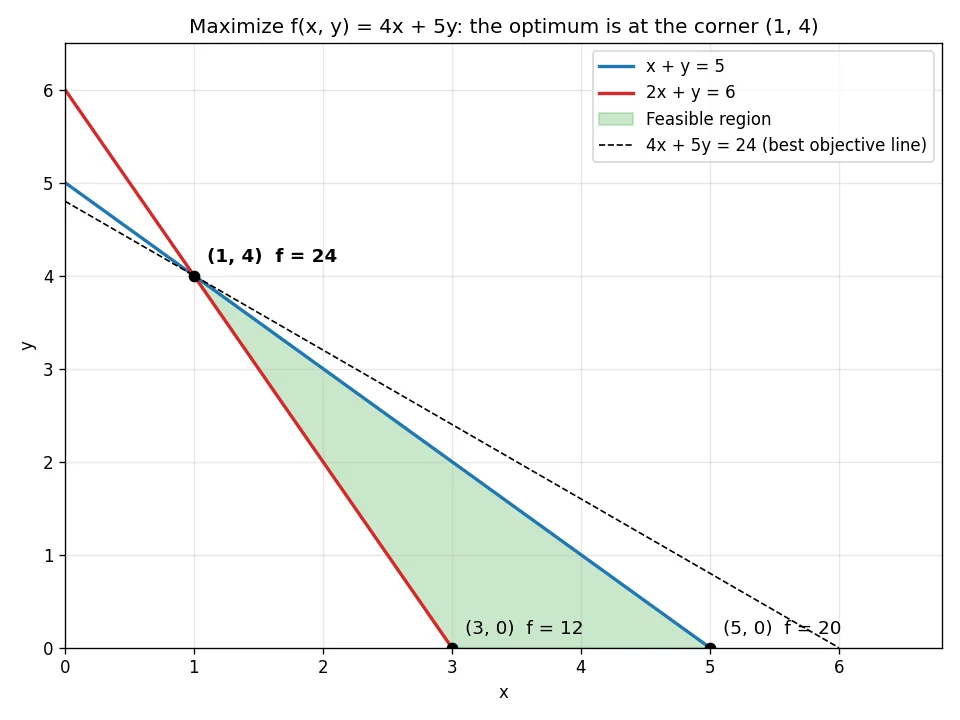
Step 2, find the corner points. Two corners lie on the x-axis: (3, 0) and (5, 0). The third is where the two lines meet: subtracting x + y = 5 from 2x + y = 6 gives x = 1, so y = 4. Note that (0, 5) is not a corner, because 2(0) + 5 = 5 is less than 6, so it breaks the second constraint.
Step 3, evaluate the objective at each corner.
| Corner (x, y) | f = 4x + 5y |
|---|---|
| (3, 0) | 12 |
| (5, 0) | 20 |
| (1, 4) | 24 |
The maximum is 24 at (1, 4). The dashed line in the graph is 4x + 5y = 24: it touches the feasible region only at that corner, which is the visual proof that no feasible point does better.
The same problem in Python with SciPy’s linprog, which minimizes and only accepts “less than or equal to” constraints, so we negate the objective and the second constraint:
from scipy.optimize import linprog

# Maximize 4x + 5y  ->  linprog minimizes, so negate the objective
c = [-4, -5]
# x + y <= 5        ->   1x + 1y <= 5
# 2x + y >= 6       ->  -2x - 1y <= -6
A_ub = [[1, 1], [-2, -1]]
b_ub = [5, -6]
bounds = [(0, None), (0, None)]  # x >= 0, y >= 0

res = linprog(c, A_ub=A_ub, b_ub=b_ub, bounds=bounds, method="highs")
print("x, y =", res.x.round(4))       # x, y = [1. 4.]
print("max value =", round(-res.fun, 4))  # max value = 24.0
I ran both Python examples with SciPy 1.13 and they print the results shown in the comments.
Nonlinear Programming
When the objective or a constraint is nonlinear (squares, products of variables, exponentials and so on), the problem is a nonlinear program. The box problem above is a simple one. The big difference from linear programming is that a nonlinear problem can have several local optima: points that are better than everything nearby but not the best overall (the global optimum).
Here is gradient descent, the method behind most machine learning training, run on f(x) = x⁴ − 4x² + x, which has two valleys of different depths:
def f(x):
    return x**4 - 4 * x**2 + x       # non-convex: two valleys of different depth

def df(x):
    return 4 * x**3 - 8 * x + 1      # derivative of f

def gradient_descent(x, lr=0.01, steps=1000):
    for _ in range(steps):
        x -= lr * df(x)              # step downhill
    return x

for start in (2.0, -2.0):
    x = gradient_descent(start)
    print(f"start {start:>4}: x = {x:.3f}, f(x) = {f(x):.3f}")

# start  2.0: x = 1.347, f(x) = -2.619   <- local minimum
# start -2.0: x = -1.473, f(x) = -5.444  <- global minimum
Starting from x = 2, gradient descent settles in the shallower valley and stops, because every small step from there goes uphill. Only the start at x = −2 finds the global minimum. This is why nonlinear problems are usually solved with several starting points or with methods designed to escape local optima.
The exception is convex problems, where the objective curves upward everywhere and the feasible region has no dents. In a convex problem, any local minimum is also the global minimum, which is why so much of practical optimization tries to formulate problems in convex form.
Common Methods for Nonlinear Problems
- Gradient descent and its variants (momentum, Adam): repeatedly step in the direction that decreases the objective fastest.
- Newton and quasi-Newton methods (such as BFGS): also use curvature information, so they usually need far fewer steps near a solution.
- Lagrange multipliers and the KKT conditions: the calculus tools for handling constraints, used inside methods such as sequential quadratic programming (SQP).
- Metaheuristics: simulated annealing, genetic algorithms, particle swarm optimization and differential evolution search widely and accept occasional worse moves to avoid getting stuck. They do not need derivatives but cannot prove that an answer is optimal.
Optimization Problems in Algorithms (DAA)
In computer science and in a Design and Analysis of Algorithms course, an optimization problem asks for the best solution among a finite (but often huge) set of candidates, like the shortest path in a graph or the most valuable set of items that fits in a bag. It is usually contrasted with a decision problem, which only asks a yes/no question such as “is there a solution with value at least k?”. Complexity classes such as NP are defined for decision problems, and an optimization problem is called NP-hard when solving it would also solve an NP-complete decision problem.
Two classic strategies for these problems are:
- Greedy algorithms make the locally best choice at each step. They are fast and correct for some problems, such as the fractional knapsack problem and minimum spanning trees (Prim’s and Kruskal’s algorithms), but they can miss the optimum elsewhere.
- Dynamic programming breaks a problem into overlapping subproblems, solves each once and combines the results. It works when the problem has optimal substructure: the best solution is built from best solutions to smaller subproblems.
Worked Example 3: Greedy vs Dynamic Programming on the 0/1 Knapsack
In the 0/1 knapsack problem, each item is taken whole or left behind, and you want the highest total value within a weight limit. With a capacity of 50 and three items:
items = [("A", 10, 60), ("B", 20, 100), ("C", 30, 120)]  # (name, weight, value)
capacity = 50

def knapsack(items, capacity):
    best = [0] * (capacity + 1)          # best[w] = best value with weight limit w
    for _, weight, value in items:
        for w in range(capacity, weight - 1, -1):
            best[w] = max(best[w], best[w - weight] + value)
    return best[capacity]

def greedy(items, capacity):
    total, left = 0, capacity
    for _, weight, value in sorted(items, key=lambda i: i[2] / i[1], reverse=True):
        if weight <= left:
            total, left = total + value, left - weight
    return total

print("dynamic programming:", knapsack(items, capacity))   # 220
print("greedy by value/weight:", greedy(items, capacity))  # 160
Greedy takes A and B, which have the best value per unit of weight, and then C no longer fits, for a total of 160. Dynamic programming finds that B and C together (weight 50, value 220) are better. If you could take fractions of items, the greedy answer would be optimal; with whole items, it is not.
Other optimization problems you will meet in algorithms courses include shortest paths (Dijkstra, Bellman-Ford), minimum spanning trees, job scheduling and the travelling salesman problem, often solved with backtracking or branch and bound when no efficient exact method is known.
Where Optimization Problems Show Up
| Field | Variables | Objective | Constraints |
|---|---|---|---|
| Logistics | Routes and loads | Minimize distance or cost | Vehicle capacity, delivery windows |
| Manufacturing | Units of each product | Maximize profit | Machine hours, materials |
| Finance | Portfolio weights | Minimize risk for a target return | Budget, position limits |
| Machine learning | Model weights | Minimize prediction error (loss) | Often none, or regularization |
| Engineering | Dimensions, materials | Minimize weight or cost | Strength, safety limits |
| Scheduling | Who does what and when | Minimize total time or overtime | Availability, precedence |
Tools for Solving Optimization Problems
- Python: scipy.optimize for linear and smooth nonlinear problems, CVXPY for convex problems, and Google OR-Tools for routing, scheduling and integer problems.
- MATLAB: the Optimization Toolbox.
- Spreadsheets: Excel’s Solver add-in handles small linear and nonlinear models.
- Commercial and open-source solvers: HiGHS, Gurobi, CPLEX and others for large linear and mixed-integer problems.
Conclusion
Every optimization problem comes down to choosing variables to make an objective as good as possible within constraints. Once you can write a problem in that form, its type tells you how to solve it: calculus for simple smooth problems, the graphical or simplex method for linear programs, gradient-based methods for nonlinear ones, and algorithms such as dynamic programming for discrete problems. The hardest part is usually the first step: writing the objective and the constraints correctly.
FAQs
What is an optimization problem in simple words?
It is the problem of finding the best choice among all allowed choices: the values that make something as large as possible (like profit) or as small as possible (like cost), while respecting limits such as a budget or capacity.
What are the three components of an optimization problem?
Decision variables (what you can change), an objective function (what you want to maximize or minimize) and constraints (the rules a valid solution must satisfy).
What are the main types of optimization problems?
Linear programming, integer and mixed-integer programming, nonlinear programming, convex optimization and combinatorial (discrete) optimization. Problems can also be constrained or unconstrained, single- or multi-objective, and deterministic or stochastic.
How do you solve an optimization problem in calculus?
Write the quantity to optimize as a function of one variable using the constraints, find where its derivative is zero, then check those critical points and the endpoints of the allowed interval to see which gives the maximum or minimum.
What is the difference between a local and a global optimum?
A local optimum is better than all nearby points; the global optimum is the best point overall. Nonlinear problems can have many local optima, but in convex problems every local minimum is also the global minimum.
What is the difference between an optimization problem and a decision problem?
An optimization problem asks for the best solution, such as the shortest route. A decision problem asks a yes/no question, such as whether a route shorter than k exists. Complexity classes like NP are defined for decision problems.
Is linear programming an optimization problem?
Yes. Linear programming is the class of optimization problems in which the objective and all constraints are linear. It is solved with the simplex method or interior-point methods, or graphically when there are two variables.